This bio-recipe explains what a linear classification (or a linear discrimination) is and shows how to compute them using Darwin. It also explains some of the algorithms used for the computation and how to gain some confidence on the results.
Classification in our definition aims to assign observations into classes. This can be used to establish a rule (a classifier) to assign a new observation into a class. In other words, previously know information is used to define the classifier and classification deals with assigning a new point in a vector space to a class separated by a boundary. Linear classification provides a mathematical formula to predict a binary result. This result is typically a true/false (positive/negative) result but it could be any other pair of characters. Without loss of generality we will assume that our result is a boolean variable, that is it takes the values true/false. To do this prediction we use a linear formula over the given input data, from here on referred to as inputs. Other names for inputs are predictors, independent variables and source variables. The linear form is computed over the inputs and its result is compared against a basis constant. Depending on the result of the comparison we predict true/false. In terms of equations this can be stated as the discriminator:
where a1, a2, ... are the variables corresponding to one observation and x1, x2, ... together with x0 are the solution vector plus basis constant. Corresponding to each input vector a there is a dependent boolean variableb. This is from now on called the output. Other terms for the outputs is responses, dependent variable and target variables. Normally we have many (m) data points (a row vector a of inputs and a corresponding output b). It is convenient to place all these data in matrices and vectors as it is the practice in linear algebra. A will denote the matrix of the inputs, A is of dimension m by n. The m boolean outputs will be stored in a vector B. The problem of linear classification can be stated now in terms of these matrices and vectors as: find x and x0 such that
The equivalence is understood as follows, every row of the left-hand-side is a relation, which for the given data will be true/positive or false/negative. This has to match the corresponding B value. In Statistics, linear classification is sometimes also called linear discrimination or supervised learning.
In general, depending on the data, or as soon as we have more data points than columns (m > n) the problem does not have a solution. That is, we cannot find a vector x that satisfies all the true values. In this case we try to find a solution which matches the vector B as "best" as possible. Best matching means either a minimum number of errors, or a weighted minimum of errors (usually a weight is assigned to the true errors and another weight is assigned to the false errors).
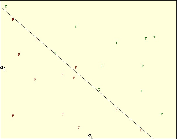
The main idea of obtaining a good classification is to be able to use it to predict the output for other (new) data points. In this context, the discriminator is a prediction formula or a model, A and B are the training data and x, x0 are the parameters of the model fitted to the training data. The following picture shows an example of the main components of linear classification:
where the true (positives) are marked with a green "T" and the false (negatives) are marked with a red "F". The inputs has two independent variables, a1 and a2 called features, which we use to position the points in the plane. There are 11 positives and 12 negatives. A linear classification in two dimensions will be a straight line. In this case the straight line drawn is a very good classification, it separates most of the points correctly. In particular, all the positives are on one side and all the negatives but one are on the other side. So this classification has one "false positive" and no "false negatives". (A false positive is a data point which is classified as positive and it is negative and conversely for false negatives.)
Classical examples of linear classification problems are medical diagnosis problems: we have individual data for a large number (m) of patients; some patients develop some particular disease, some don't. The purpose of classification in this case is to find a linear formula on the data of the patient that can describe the condition (diseased/healthy). Once that we have found a classification, we must validate it. This means testing that it has predicting power, and how accurate it appears to be. Notice that finding a good classification does NOT guarantee that it will be a good predictor.
Finally, if the outputs are numerical i.e. it is not binary, then classification is not appropriate. See function approximation (SVD, BestBasis, etc.) for that purpose.
Darwin has a main function to compute linear classifications called "LinearClassify". The information computed is stored in a class called "LinearClassification".
?LinearClassify
Function LinearClassify - Linear form which does pos/neg classification

Calling Sequence:  LinearClassify(A,accept,mode,WeightNeg)

Parameters:
  Name        Type               Description
  -----------------------------------------------------------------------------
  A           matrix(numeric)    an n x m matrix of independent variables
  accept      {list,procedure}   positive/negative determination
  mode        anything           optional, algorithm selection, defaults to Svd
  WeightNeg   positive           optional, weight of negatives

Returns:
	LinearClassification
Synopsis:  Computes a vector X such that the values A[i]*X >= X0 classify the
  positive/negatives.  Such a vector is called a linear discriminant in
  statistics.  A special way of computing such a vector is called the Fisher
  linear discriminant.  LinearClassify normally produces results which are
  much better than the Fisher linear discriminant.  LinearClassify returns a
  data structure called LinearClassification which contains the vector X and
  the splitting value, called X0, the weights of positive and negatives, the
  score obtained and the worst mis-classifications.  The third argument, if
  present, directs the function to use a particular method of computation.
  The methods are
  mode           description
  -------------------------------------------------------------------------
  BestBasis      equivalent to BestBasis(10)
  BestBasis(k)   Least Squares to 0-1 using SvdBestBasis of size k
  Svd            (default mode) equivalent to Svd(1e-5)
  Svd(bound)     Least Squares to 0-1 using Svd, with svmin=bound
  Svd(First(k))  LS to 0-1 using Svd so that k sing values are used
  CenterMass     Direction between the pos/neg center of masses
  Variance       Variance Discrimination of each variable
  Fisher         Fisher linear discriminant
  Logistic       Steepest descent optimization using the logistic function
  CrossEntropy   Steepest descent optimization using cross entropy
  Best           equivalent to Best(10)
  Best(n)        A combination of methods found most effective by
                 experimentation.  n determines the amount of optimization.
  <default>      Svd(1e-5)
 In practice the best results are obtained with Best(n).  Svd(1e-12) and
  CrossEntropy are also very effective.  Once a LinearClassification has been
  computed, it can be improved or refined with the functions:
     function                      description
     --------------------------------------------------------------------
     LinearClassification_refine   find the center of the min in each dim
     LinearClassification_refine2  Svd applied to a hyperswath
     LinearClassification_refine3  Minimize in a random direction
     LinearClassification_refine4  Svd on progressively smaller swaths
Unless you use the Best option, no matter how good the initial results are, it
  always pays to do some refinement steps.  In particular refine2 and refine4
  give very good refinements.

Examples:
> A := [[0,3], [8,5], [10,7], [5,5], [7,4], [7,9]]:
> lc := LinearClassify( A, [0,1,1,0,1,0] ):
> print(lc);
solution vector is X = [0.1945, -0.1364]
  discriminator is A[i] * X > 0.553293
6 data points, 3 positive, 3 negative
positives weigh 1, negatives 1, overall misclassifications 0
Highest negative scores: []
Lowest positive scores: []
See Also:
             ?LinearClassification    ?Stat           ?SvdBestBasis
             ?LinearRegression        ?SvdAnalysis


   ------------
?LinearClassification
Class LinearClassification - results of a linear classification

Template:  LinearClassification(X,X0,WeightPos,WeightNeg,NumberPos,NumberNeg,
                WeightedFalses,HighestNeg,LowestPos)

Fields:
  Name             Type                      Description
  ----------------------------------------------------------------------
  X                list(numeric)             solution vector
  X0               numeric                   threshold value
  WeightPos        numeric                   weight of the positives
  WeightNeg        numeric                   weight of the negatives
  NumberPos        posint                    number of positives
  NumberNeg        posint                    number of negatives
  WeightedFalses   numeric                   weighted misclassifications
  HighestNeg       list([posint, numeric])   highest scoring negatives
  LowestPos        list([posint, numeric])   lowest scoring positives

Returns:
	LinearClassification
Methods:   DirOpt2   DirOpt3   DirOpt4   print   refine   type
Synopsis:  Data structure which holds the result of a linear classification.
  A linear classification is defined by a vector X, such that the internal
  product of every data point A[i] with X can be compared against a threshold
  and decide whether the data point is a positive or a negative.  I.e. A[i] X
  < X0 implies a negative and A[i] X >= X0 a positive.
See also:  ?LinearClassify


   ------------
User who are only interested in using this function, should ignore all the choices for mode and use "Best". This uses a very effective combination of optimizations. The examples in the next two sections will also be useful for the practitioner.
Notice that finding a linear classification is a very difficult problem. It is NP-complete when the matrix A is composed of 0's and 1's. (The two-dimensional example is misleadingly simple, in higher dimensions it becomes basically intractable.) So our algorithms are going to be approximate by force.
The following example shows how to construct data that has a desired level of classification. We can submit this data to our function and see how well it does in discovering the relations. Synthetic examples are excellent to test the quality of the algorithms for linear classification. Real data is interesting for other obvious reasons, but when we want to evaluate how the algorithms to find classifications perform, it should be with synthetic data of this nature.
We will use a matrix A of random normally distributed numbers.
m := 100;  n := 10;
A := CreateArray( 1..m, 1..n ):
for i to m do for j to n do A[i,j] := Rand(Normal) od od:
# print 3 rows, to see if they are ok
print( A[1..3] );
m := 100
n := 10
 -1.3202 -0.6293  0.5911  0.0651 -0.0350  0.0246 -1.9268  0.1629 -0.2779 -0.3022
 -0.1996  0.1359  1.3616  2.4518  0.0184 -1.4088 -0.8077 -0.0589 -2.4263 -0.8450
 -0.0705 -0.6531 -1.1668  0.6330 -0.5435  1.6289 -0.1584 -0.6618  0.1331 -0.6210
Now we have to decide which is going to be our linear relation. Once that we have it, we use it to compute the vector B. We can do this deterministically or adding some noise. For this example we will add random noise. We will also compute how many entries are correct under our (known) linear formula.
B := CreateArray( 1..m ):
for i to m do B[i] := 3*A[i,3] - 4*A[i,5] + Rand() > 0.1 od:
# print the first 3 to check
print( B[1..3] );
correct := 0:
for i to m do
    if ( 3*A[i,3] - 4*A[i,5] > 0.1 ) = B[i] then
	correct := correct+1 fi
od;
lprint( correct );
[true, true, false]
99
Now we are ready to compute the linear classification:
lc := LinearClassify( A, B, Best ):
print(lc);
solution vector is X = [-0.7431, -0.6004, 7.2707, 0.5679, -10, -0.6192, -0.3624, -1.6222, -0.6198, -0.1855]
  discriminator is A[i] * X > -0.731373
100 data points, 39 positive, 61 negative
positives weigh 1, negatives 0.639344, overall misclassifications 0
Highest negative scores: []
Lowest positive scores: []
At first glance the results appear very different from the expected, but this is not so. The solution vector accepts an arbitrary scaling, and it is scaled so that its largest component be 10 in absolute value. If we scale it back, we find:
lc[X] * 4/10;
[-0.2972, -0.2402, 2.9083, 0.2272, -4, -0.2477, -0.1450, -0.6489, -0.2479,
-0.07419078]
and we can see that the main components are the third and the fifth and they have the right values. The rest of the differences can be explained by the fact that the noise that we added was probably too large, and our formula produced 1 errors. The classification found by the program has 0 misclassifications, so it is clearly better. The rest of the columns were used to compensate for the extra noise.
We can now use the linear classification to predict the output b for a new randomly generated point
new:=[]:
to n do new:=append(new, Rand()) od:
new*lc[X]>=lc[X0];
false
We will now run a more realistic example based on properties of proteins. Our goal is to derive a classification scheme that can determine if a protein is an outer membrane protein or not. To do this we will use the data in SwissProt, which we have to load first. We will search for the string "outer membrane" in the entire database with the command SearchDb.
SwissProt := '~cbrg/DB/SwissProt.Z':
ReadDb(SwissProt):
memb := [SearchDb('outer membrane')]:
lm := length(memb);
Reading 169638448 characters from file /home/cbrg/DB/SwissProt.Z
Pre-processing input (peptides)
163235 sequences within 163235 entries considered
lm := 942
There are 942 matching sequences. This is a good size for our sample. Next we should select a similar size sample with entries which are not membrane proteins. We will do this by selecting random entries from the database and requiring that the word "membrane" does not appear in their definition (notice that SearchString returns -1 when it does not match).
non_memb := []:
while length(non_memb) < lm do
    e := Rand(Entry);
    if SearchString( membrane, e ) < 0 then
         non_memb := append(non_memb,e) fi
od:
As features we will use the amino acid frequencies of these sequences. This will give us 20 values per protein. Technically, all the frequencies add to 1, so we need only 19, but it does little harm to linear classification to have extra variables. We concatenate the membrane entries followed by the non-membrane entries and then compute the amino acid frequencies for all of them. We will place this information in the matrix A. We write a function to compute the amino acid frequencies of a given entry.
AAFreq := proc( e )
    F := CreateArray(1..20);
    s := Sequence(e);
    for i to length(s) do
		j := AToInt(s[i]);
		if j > 0 and j < 21 then F[j] := F[j]+1 fi
	od;
    F / sum(F)
end:
A := [ seq( AAFreq(i), i = [ op(memb), op(non_memb) ] )]:
We are almost ready to compute the classification, we just need to construct the vector B, which in this case will have its first half filled with "true" and its second half with "false".
B := [seq(true,i=1..lm), seq(false,i=1..lm)]:
lc2 := LinearClassify( A, B, Best ):
print( lc2 );
solution vector is X = [2.3323, -1.5549, 2.7910, -0.3047, -9.8599, 3.3371, -4.3826, 0.3360, -8.9198, -2.7926, -0.2509, 0.1157, -2.8817, -1.6977, -4.9915, 3.2286, 2.3616, 10, 3.5917, 0.05464701]
  discriminator is A[i] * X > -0.000236669
1884 data points, 942 positive, 942 negative
positives weigh 1, negatives 1, overall misclassifications 302
Highest negative scores: [[1.5261, 1464], [1.0716, 1718], [1.0574, 1726], [1.0468, 1509], [1.0177, 1374], [0.9426, 1023], [0.8751, 1355], [0.8003, 1112], [0.7304, 1815], [0.7025, 1883], [0.6449, 1669], [0.6324, 1053], [0.6042, 1423], [0.5885, 1339], [0.5798, 1201], [0.5740, 1719], [0.5281, 1124], [0.5250, 1501], [0.5205, 1829], [0.5188, 1824]]
Lowest positive scores: [[-1.7366, 462], [-1.6998, 459], [-1.5951, 463], [-1.5743, 460], [-1.5443, 461], [-0.9745, 803], [-0.9461, 804], [-0.9185, 381], [-0.9105, 805], [-0.6499, 806], [-0.6129, 252], [-0.5489, 485], [-0.5421, 881], [-0.4941, 486], [-0.4894, 91], [-0.4893, 56], [-0.4880, 235], [-0.4811, 930], [-0.4659, 271], [-0.4552, 321]]
This appears to be a mediocre classification with 302 misclassifications. We print a table with the coefficients of the classification for each amino acid. Remember that the coefficients are multiplied by the frequency of the amino acid to evaluate the discriminator. So a positive coefficient means that abundance of that amino acid suggest being and "outer membrane" protein. A negative coefficient, the converse. The magnitude of the coefficients indicate their relative importance.
for i to 20 do
    printf( '%s  %6.2f\n', IntToAAA(i), lc2[X,i] ) od;
Ala    2.33
Arg   -1.55
Asn    2.79
Asp   -0.30
Cys   -9.86
Gln    3.34
Glu   -4.38
Gly    0.34
His   -8.92
Ile   -2.79
Leu   -0.25
Lys    0.12
Met   -2.88
Phe   -1.70
Pro   -4.99
Ser    3.23
Thr    2.36
Trp   10.00
Tyr    3.59
Val    0.05
Naturally, this is just a first approximation, if we were to pursue membrane classification we should add more features which may be related with the property in the hope of improving the results.
We will now use the linear classification for membrane proteins to see if it will correctly assign another membrane protein.
new:=AAFreq(Entry(4799)):
new*lc2[X]>=lc2[X0];
false
Lets try the same for a non-membrane protein
new:=AAFreq(Entry(1801)):
new*lc2[X]>=lc2[X0];
false
In this section we give a very brief overview of the main problems/ideas behind the algorithms for computing linear classifications. There are many books and papers written on the subject, far too many to cover here. The algorithms for finding good linear classifications typically have 3 components:
| A | An initial solution |
| B | A refinement procedure to improve solutions |
| C | A method to introduce some randomness. |
The construction of the initial solution consists of the vector x and x0. As it turns out to be, computing x0 is not very difficult, it just requires the sorting of the vector Ax plus an additional linear pass. So the difficulty of the problem lies in the computation of the direction x. The refinement algorithms, if they have some randomness, can be applied repeatedly and hence produce better solutions. As we have various refinements algorithms, we can also alternate with the different refinements.
The different methods are described in detail and are complemented with extensive simulation results. One clear conclusion is that none of the methods to build an initial classification is uniformly better than the others. As a matter of fact, they all pale against an arbitrary method and a few steps of refinement.
It should be noticed that the linear discriminator de facto includes a constant term. So adding a constant term in the input variables is of no use.
A linear classification remains unchanged if it is multiplied by an arbitrary positive constant. (all the coefficients in x and x0 are multiplied by the same constant.) To make results more readable and comparable, it is customary to normalize the result, so that the norm has some property. Darwin chooses to make the largest component of x equals to 10 in absolute value.
Similarly, multiplying a particular input variable by an arbitrary constant has no effect (the corresponding value of x is divided by this constant). Adding an arbitrary constant to an input variable has no effect either, its value is absorbed by the constant x0. So we can apply a linear transformation of the input variables without any harm on the linear classification itself. In this case, it is sometimes reasonable to transform all input variables so that they have average 0 and variance 1. A secondary effect of this transformation is that the magnitudes of the x values are now comparable.
A primitive form of non-linear classification can be obtained by including the input variables and some of their powers, for example their squares. The benefits of this are not always positive. There is one case where this helps, which is when a classification depends on a particular input variable being inside a range. Purely linear classification will never be able to cope with a range, but including the square of the variable will produce a linear classification that resolves this problem.
© 2005 by Gaston Gonnet, Informatik, ETH Zurich
Last updated on Fri Sep 2 16:55:12 2005 by GhG